Creating an MTP set
The best way to create an MTP set (a group of microbiome samples) is to use metadata tags (shortly tags). A tag is a short word that represents a single feature of a sample. An MTP (sample) can be explained as a series of tags. For example, a sample from a 70-year-old, male, non-smoking US citizen who is an obese patient can be labeled by the following tags: [US] [senior] [male][non_smoking][obesity]. Please note that a tag does not contain a blank space character which should be replaced by an underscore (_).
Creating tags
You must create tags before you can apply them to your MTPs. You can do this by opening .
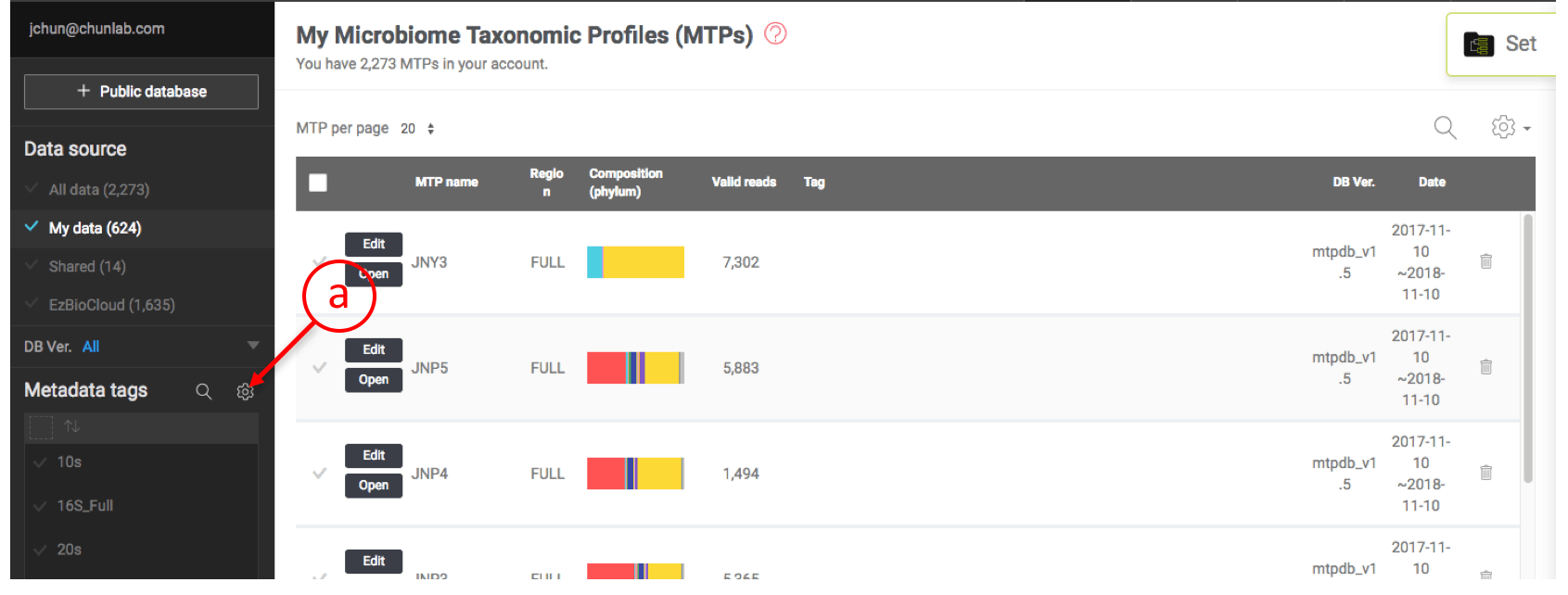
Open metadata tag manager
- Open by clicking this icon.
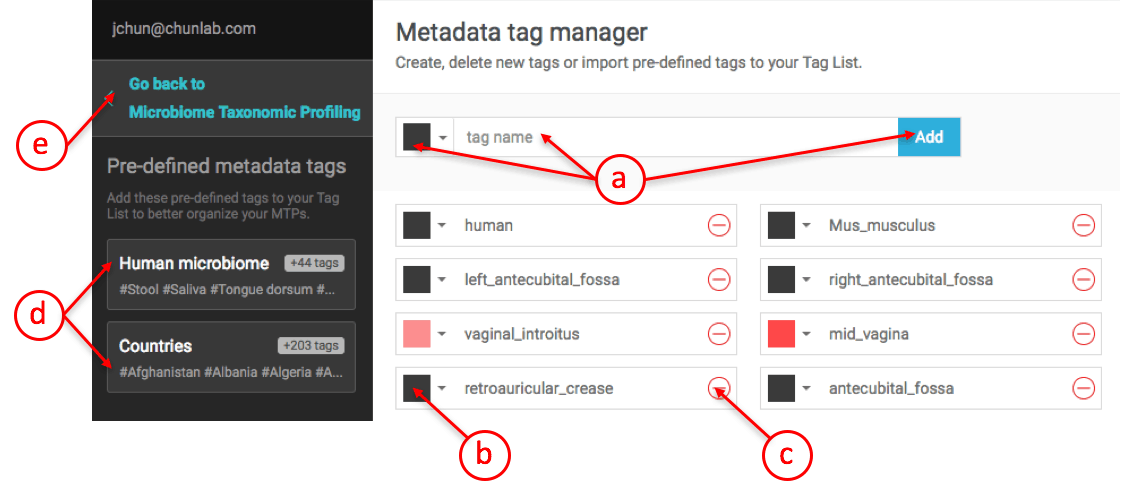
Creating metadata tags in
- Here, you can add a new tag and choose a color for it.
- You can change the color of a tag later.
- You can delete any tag later.
- These are pre-defined tags provided by the EzBioCloud team. Please use these to maximize the compatibility with the provided public datasets.
- When you finish creating or managing tags, click here to go back to the main MTP page.
Attaching the metadata tags to MTPs
After you create tags, it is now time to attach the tag(s) to each MTPs.
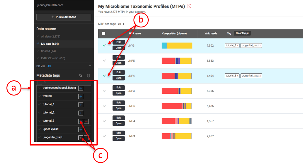
Attaching tags to MTPs
- This is the Metadata Tag Panel where you can select MTPs using a combination of tag(s).
- First, select the MTPs that you want to attach the desired tags. Here, two MTPs (JNY3, JNP4) are selected.
- Click [+] at the “tutorial_3” and “urogenital_tract” tags to attach them to the selected MTPs.
Selecting MTPs to create an MTP set
In the below screenshot, only MTPs with the tag “tutorial_3” are selected by checking/selecting “tutorial_3” at the metadata tag panel.
Selecting MTPs using a single tag (“tutorial_3”)
- This is the Metadata Tag Panel.
- Here, “tutorial_3” is selected.
- Only the MTPs with “tutorial_3” are now selected.
- Please note that the color-labeled tags are displayed with the designated colors (see the above section on “Creating tags”).
- Check this box if you want to unselect all tags.
- Search tag(s) using a search word. For example, enter “antibio” to search both “antobiotics+” and “antibiotics+”.
In the below case, two tags (“tutorial_3” and “Cdiff+”) are selected.
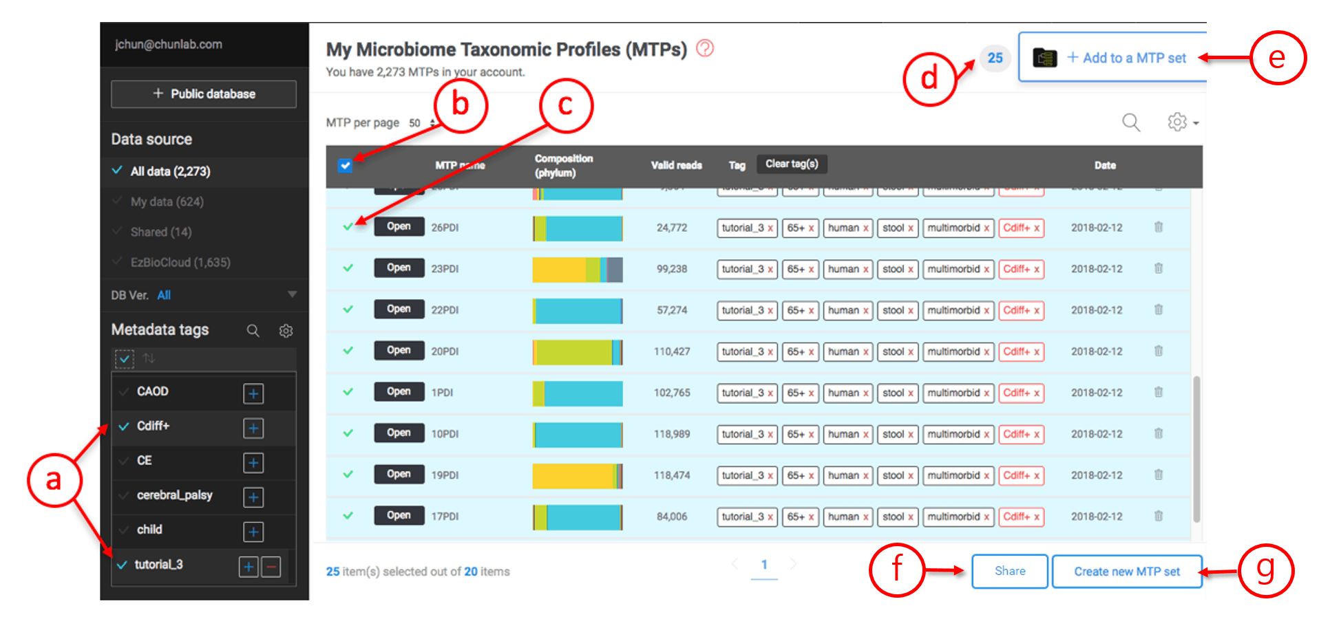
Creating an MTP set
- Two tags are selected. You can use any combinations of tags.
- Check this box to select all MTPs listed by tagging.
- Unselect or select an individual MTP.
- The number indicates the total number of MTPs selected.
- Click this tab to add the selected MTPs to an existing set.
- Click this tab to share the selected MTPs with other users.
- Click this tab to create an MTP set.
You can name an MTP set as you wish. Just remember that the set names will be used in many visualizations such as charts and scattergrams, so concise and informative names are highly recommended.
The EzBioCloud team / Last edited on Feb. 8, 2019
Browsing an MTP set
An MTP set consists of two or more MTPs, representing a group of microbiome samples. Once an MTP set is created, it can be browsed by the . Here, we will open a set called “seniors” which contains 68 MTPs with the same and different tags (For example, all MTPs has “senior” tag, but only some are labeled with “Cdiff+”, “antibiotics+” or”antibiotics-“.
Opening the MTP set browser
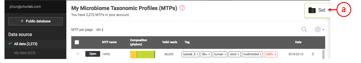
Open an MTP set
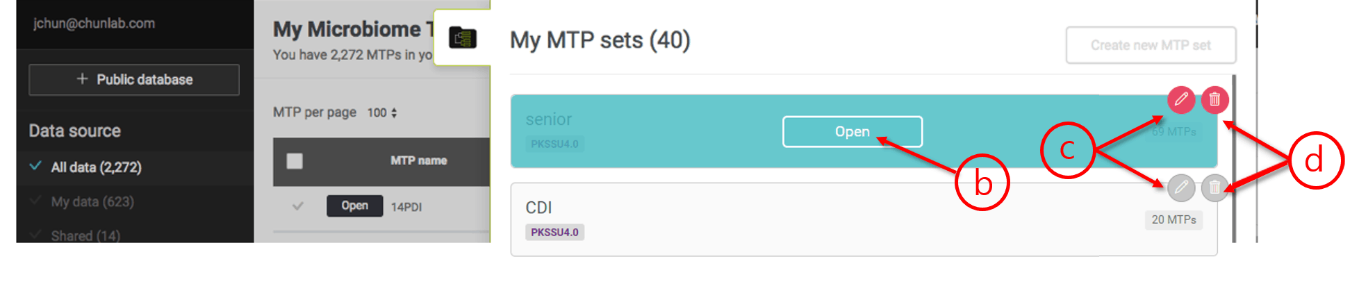
- All MTP sets are available here. You can generate an unlimited number of sets. Click the tab to bring out the list of your MTP sets.
- Open the desired MTP set.
- Edit the MTP set name of the set
- Delete the set if you want.
There are four menus in the MTP Set Browser.

Top menus of the MTP Set Browser
MTP List
In this page, the list of MTPs in the set is displayed.
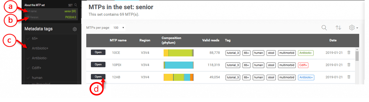
Listing MTPs in an MTP set
- Name of the MTP set
- Taxonomic database version used for the MTP pipeline. MTPs of the different versions of databases cannot be included in the same set.
- Select tag(s) to quickly filter MTPs.
- Open an MTP if you want to explore single MTP.
Composition
In this page, three submenus (tabs) are provided: , , and
Stacked bar
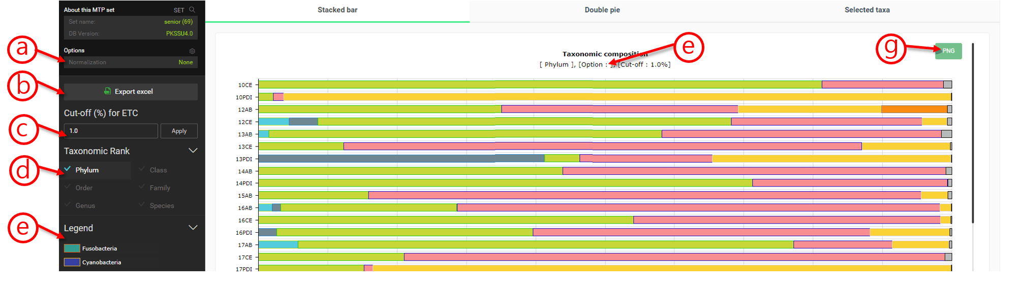
Stacked bar visualization of an MTP set
- You can change the option for normalization. You can normalize or correct the compositional data using re-sampled reads or gene copy number [Learn more].
- You can export the data as an Excel spreadsheet file.
- All reads that are present in minor quantity are classified as ETC. You can change the cut-off for the ETC reads here.
- You can select the taxonomic rank to visualize.
- Color legends are located here for the stacked bar chart.
- Parameters applied are given here.
- An image file can be downloaded here.
Double pie
The double pie chart is a special, interactive chart that simultaneously displays compositions of two taxonomic ranks in the sample time.
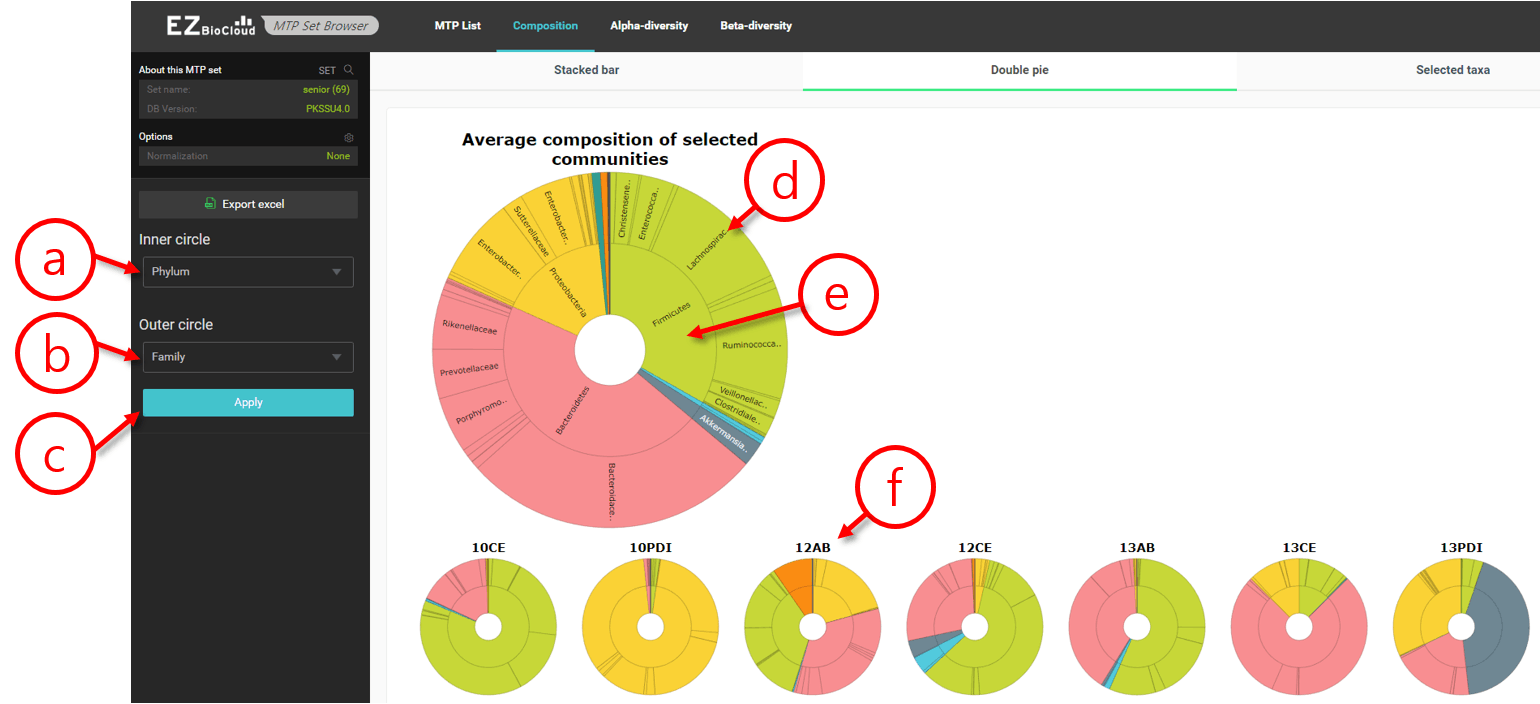
Double pie chart of an MTP set
- Select the taxonomic rank of the inner circle.
- Select the taxonomic rank of the outer circle.
- Click [Apply] to make the change effective.
- This is the outer circle for the averaged composition profiles of all MTPs in the set. Bring the cursor to highlight the taxon (pie).
- This is the inner circle.
- These are the double pie chart of individual MTPs.
Selected taxa
In this page, the composition of a selected taxon can be shown as a box plot. In addition, predefined sets are provided to quickly browse the compositional information.

Selected human gut taxa in an MTP set
- Predefined taxonomic groups are listed here. We will expand them in future.
- Here, “human gut taxa” is selected to list all important taxa of the human gut microbiome.
- Box plots are shown here [Learn more].
- By clicking this, box plots will be re-drawn with the outliers.
- An image file can be downloaded here.
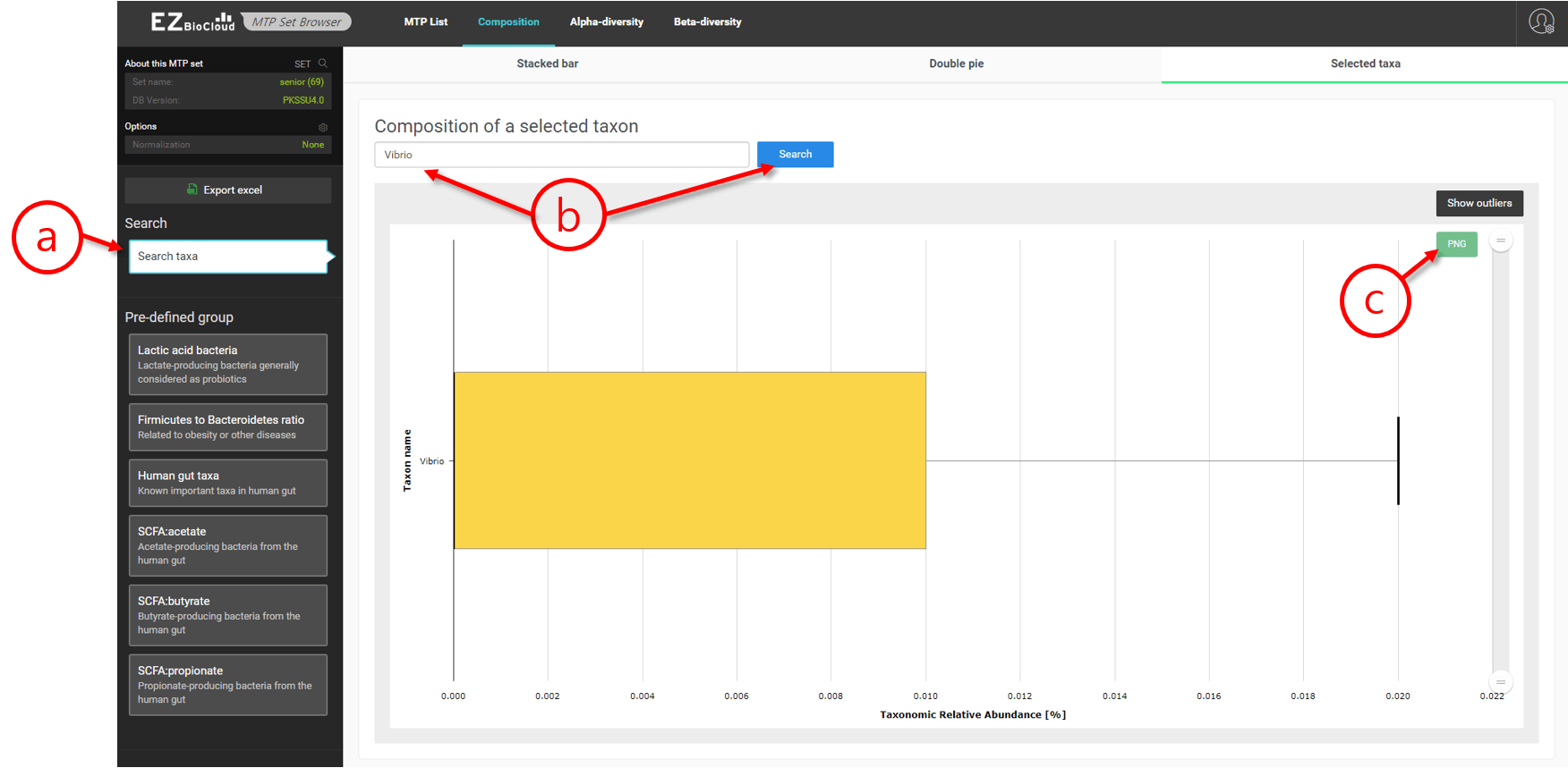
Box plot of the relative abundance of a selected taxon in an MTP set
- Enter a name of taxon here to display. You can input any taxon from phylum to species.
- In this example, “Vibrio” is entered, and the result shows that there are very little Vibrio species found in this MTP set.
- An image file can be downloaded here.
Alpha-diversity
In this menu, general information and indices explaining alpha-diversity are provided. Basically, alpha-diversity indices are calculated for each MTPs. In this visualization, all of those values are shown side by side for you to quickly compare.
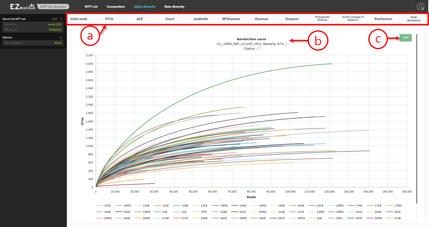
Alpha-diversity indices of an MTP set
- Various alpha-diversity indices are given in this page.
- In this screenshot, individual rarefaction curves of 69 MTPs are shown in a chart.
- Download an image of this chart.
Beta-diversity
Beta-diversity analytics allows us to understand the relationship of microbial communities stored in multiple MTPs. At present, these are presented as either ordination analysis or hierarchical clustering. The first step for the beta-diversity is to calculate the distances among the set of MTPs. In the ordination analysis, the data reduction of the distance matrix is performed by the principal coordinate analysis (PCoA) to give the major axes of principal components (PCs). In EzBioCloud 16S-based MTP app, we take either the first two or three PCs to draw the scattergrams. The same distance matrix can be used to carry out the hierarchical clustering using UPMGA algorithm (Unweighted Pair Group Method with Arithmetic Mean). There are several different algorithms to calculate beta-diversity distances and pertaining parameters. EzBioCloud 16S-based MTP app allows instant and interactive navigation of data space using optimized user interface.
PCoA (2D)

PCoA-based 2-dimensional ordination scattergram
- Select a beta-diversity distance metric.
- Decide if you want to include data up to the species or genus level.
- Some sequencing reads are not taxonomically identified at the species or higher level. These reads are assigned in the unclassified group (labeled as *_uc). You can choose to either include or exclude these data. If most of the reads were assigned to the species, which is most cases in human microbiome analysis of EzBioCloud, this option will have a very small impact on the outcome of beta-diversity.
- Time to maximize your tags here. Select a tag to quickly display the sub-set of MTPs in your MTP set. In this screenshot, the tag “Antobiotic+” was selected to highlight the MTPs (human subjects) who took the antibiotics.
- Changing or selecting a combination of tags (e.g. “Antibiotic+” and “CDiff+”) will highlight the picked MTPs (Clostridium difficile infection patients who took antibiotics) in this 2D plot.
- An image file can be downloaded here.
- Download the list of three PCoA axes as a excel format file.
PCoA (3D)
This is the same scattergram as the above 2D one, except that it takes an additional, first principle component axis.
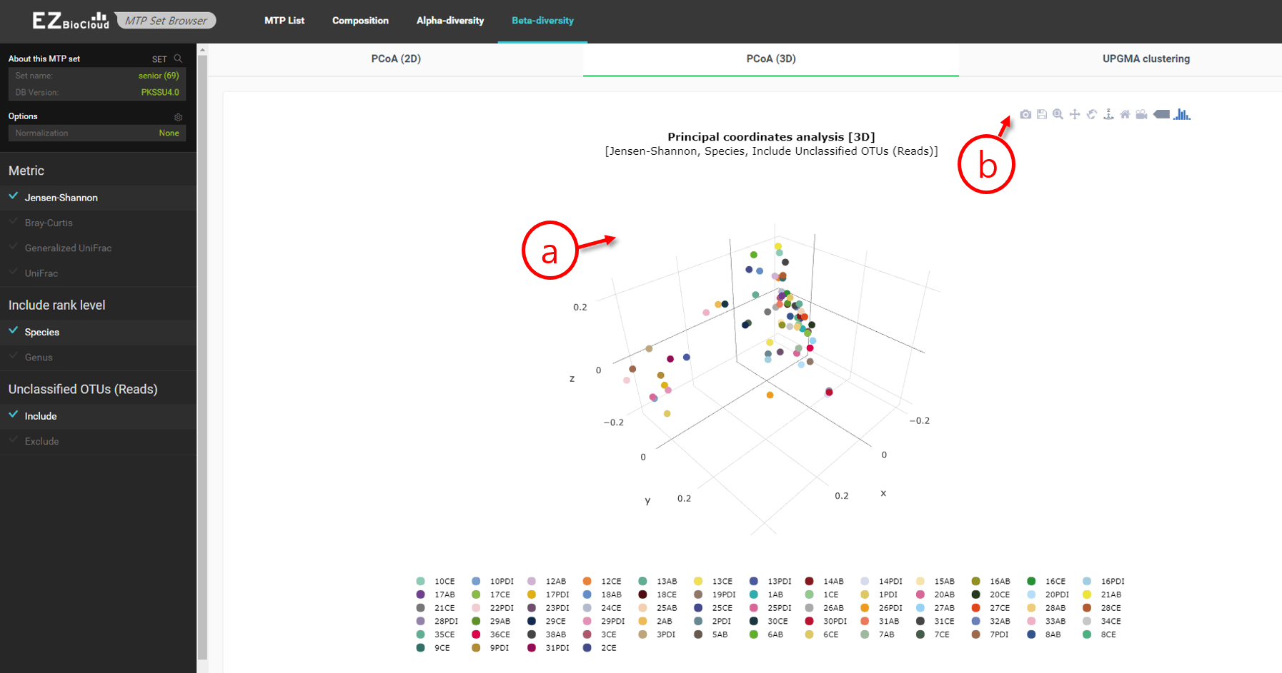
PCoA-based 3-dimensional ordination scattergram
- Use the left click+mouse to rotate the figure.
- Bring the cursor will highlight additional menus on this visualization.
UPGMA clustering
Unlike ordination diagrams, hierarchical clustering forces each MTPs (samples) to be grouped in a strictly hierarchical way. Again, you can change the distance algorithms and associated parameters. The chart should be called a dendrogram, not a phylogenetic tree.
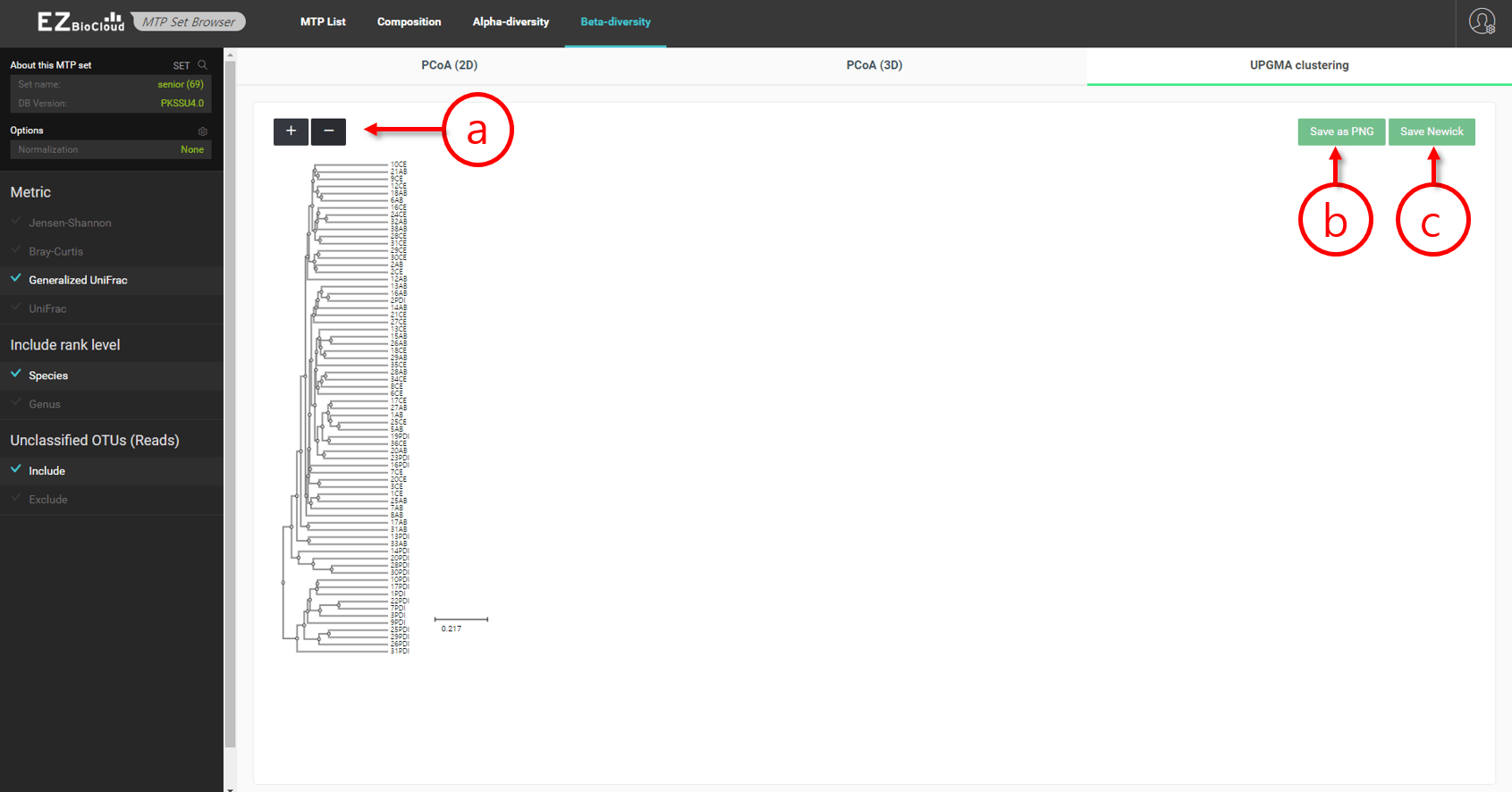
A dendrogram resulted from a UPMGA clustering
- Enlarge or reduce the dendrogram.
- Download the dendrogram as an image.
- Download the dendrogram as a Newick format file which can be read by other tree viewing software tools.
The EzBioCloud team / Last edited on Feb. 8, 2019
Starting
Microbiome samples, MTPs, are grouped into the sets and compared to find differentially present taxa. EzBioCloud 16S-based MTP app provides several ways of visualization and statistical analyses, under the menu <Comparative MTP Analyzer>. To use this functionality, you must create at least two sets of MTPs in advance [Learn more].
The function can be accessed from the
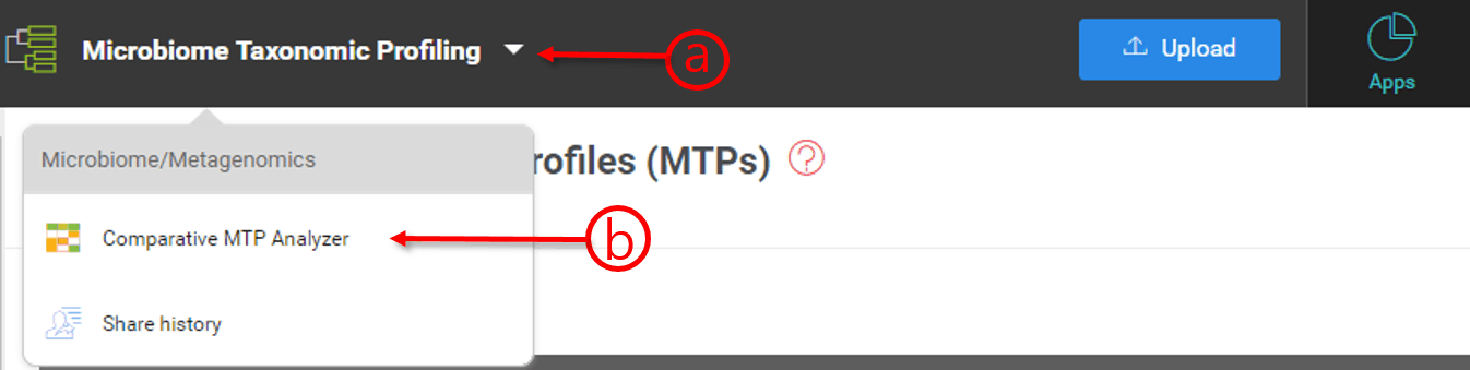
- Click here to open the pull-down menu to go to other services.
- Select
Choosing MTP sets and the comparative analytics service
You can compare up-to five MTP sets depending on your subscription model [Learn more].
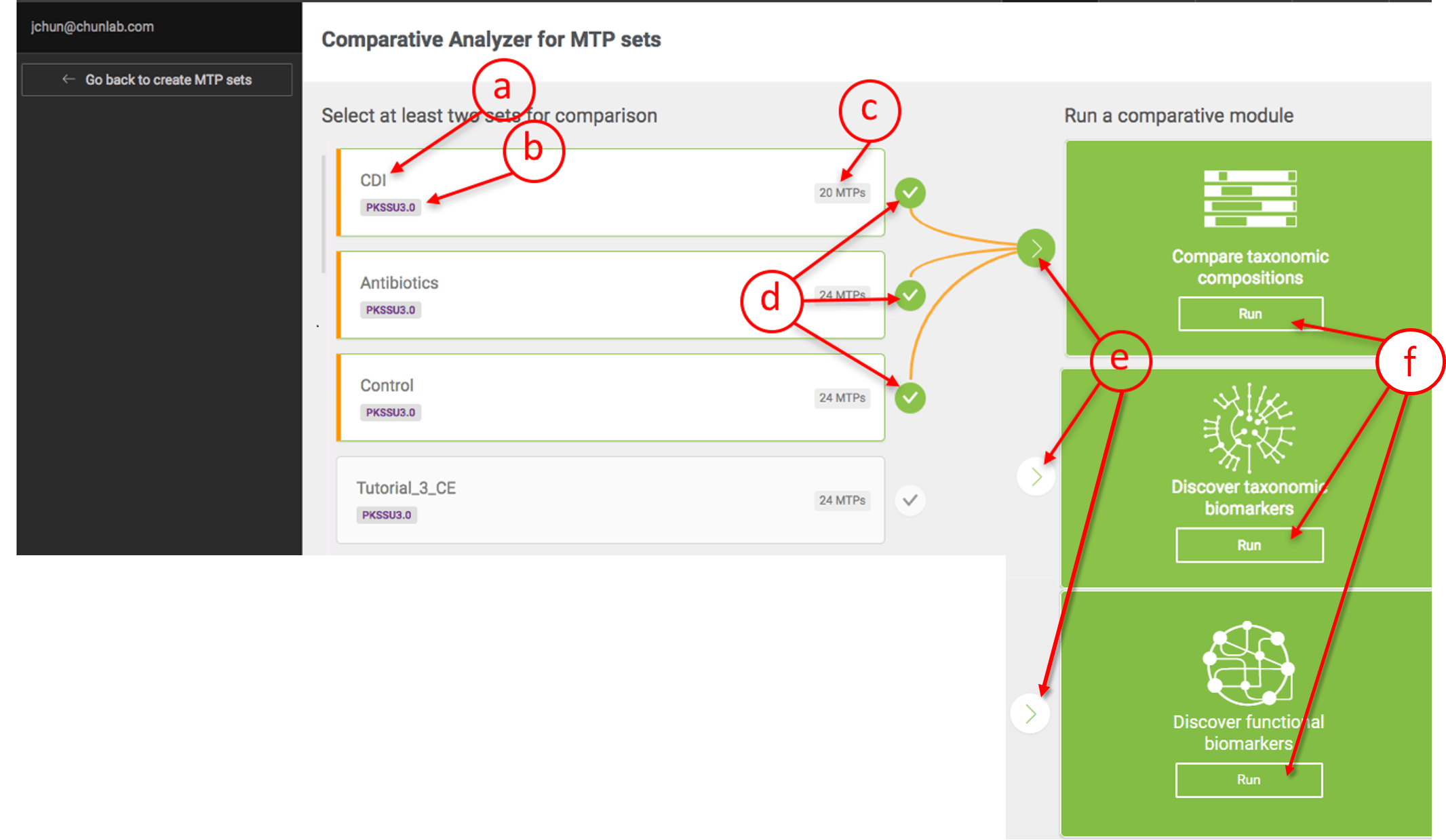
Selecting MTP sets for comparative analysis
- Name of MTP set
- The version of the taxonomic database. Only sets with the same version of the database can be compared.
- Number of MTPs in this set
- Select the desired MTP sets. In this example, three sets (CDI, Antibiotics, and Control) are selected.
- Select a comparative module.
- Then, click [Run] to launch the main page.
The order of the “set selection” is important as the sets will be displayed in that order for all subsequent visualization and analyses.
In this example, the order of selection was (1) Control, (2) Antibiotics, then (3) CDI.
The EzBioCloud team / Last edited on Feb. 8, 2019
Comparative MTP Analyzer
Comparative MTP Analyzer consists of the following functionalities.

| Composition: | Compare relative taxonomic abundances among sets. E.g., find the overall difference in taxonomic compositions between the healthy and diseased subjects. |
| Alpha-diversity: | Compare alpha-diversity indices among sets. E.g., find if a set of diseased subjects shows lesser species diversity than that of healthy subjects. |
| Beta-diversity: | Compare beta-diversity indices among sets. |
| Taxonomic biomarker discovery: | Find differentially present species that are characteristic of a disease. |
Composition
Three visualization methods are provided here.
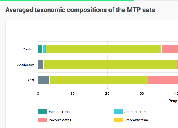
Stacked bar
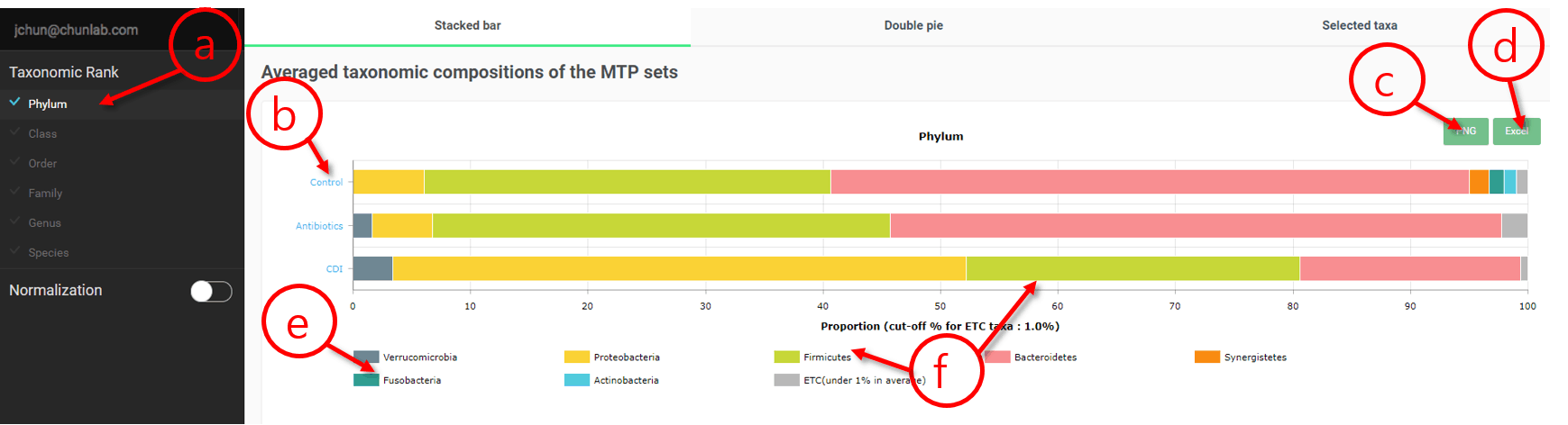
Compostional analysis in Comparative MTP Analyzer
- Select a taxonomic rank here.
- The names of MTP sets. Please note that the order of displayed sets was set when you select the sets.
- Download the chart.
- Download the taxonomic profiles.
- Click this small box to go to the page of the taxon (Fusobacteria phylum in this example).
- Click on the box or taxon name that you are interested to highlight (as shown as the below figure).
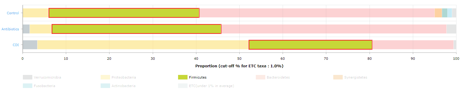
“Firmicutes” phylum was selected and highlighted.
Double pie chart
This module visualizes a pie chart showing two different taxonomic ranks simultaneously.
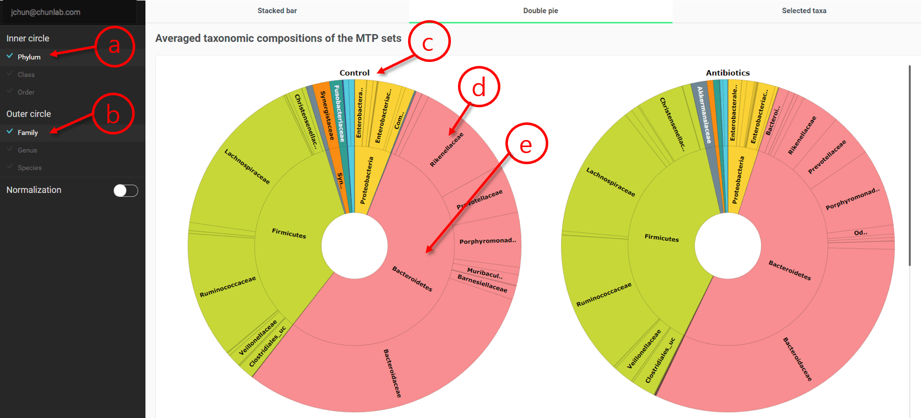
Double pie chart in Comparative MTP Analyzer
- Select a taxonomic rank for the inner circle.
- Select a taxonomic rank for the outer circle.
- Name of the MTP set
- Taxonomic composition of the outer circle, as selected in (b).
- Taxonomic composition of the inner circle, as selected in (a).
Selected taxa
In this module, the composition of the selected taxa can be shown as box plots [Learn more]. In addition, predefined sets are provided to quickly browse their compositional information.
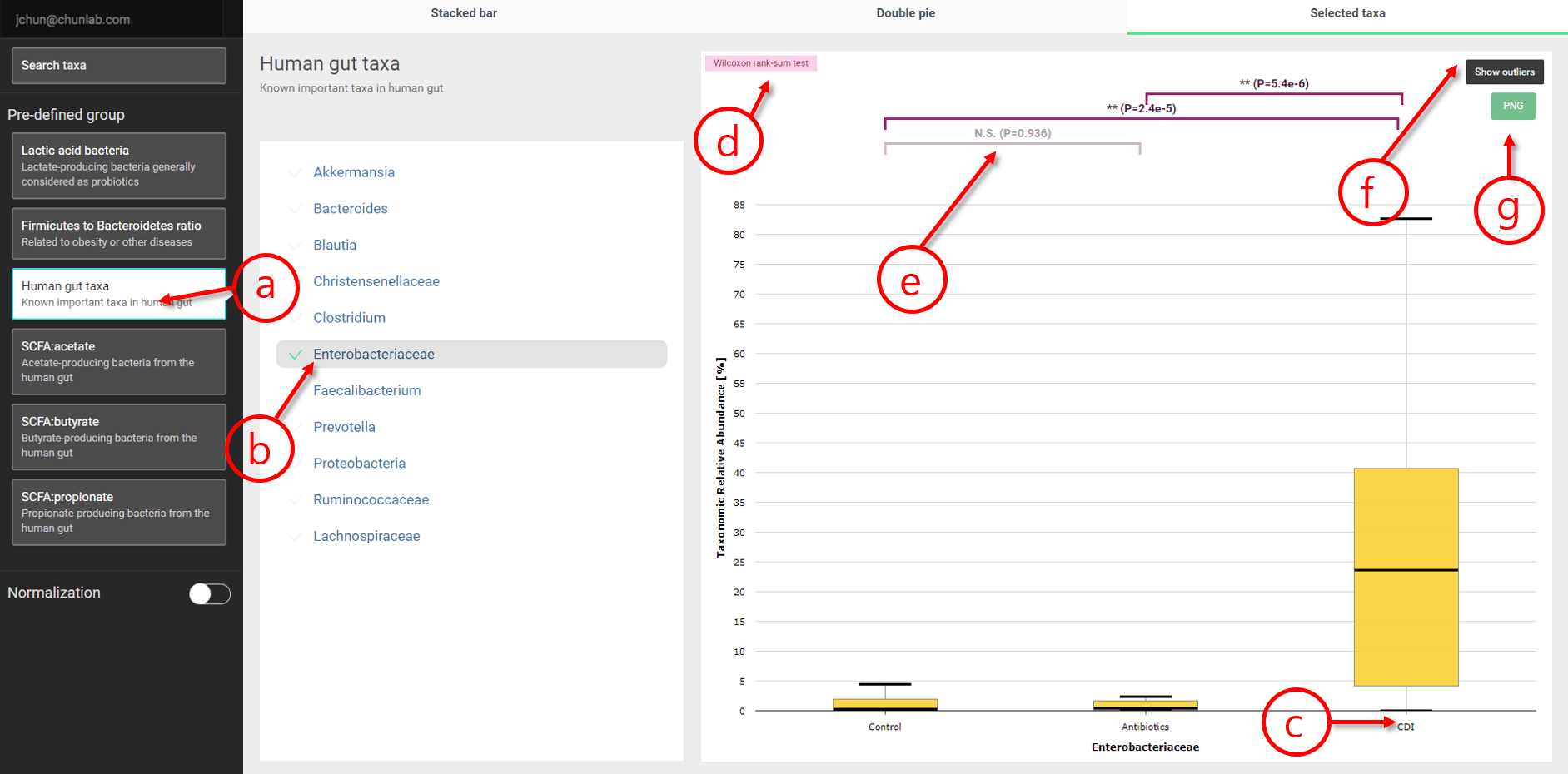
Selected taxa in Comparative MTP Analyzer
- A predefined group, “Human gut taxa”, is selected.
- Among them, “Enterobacteriaceae” is selected. This family contains Escherichia coli and is known to be associated with inflammation.
- Name of an MTP set. In this example, CDI set contain C. difficile infection-positive seniors.
- “Wilcoxon rank-sum test” is used to test the null hypothesis.
- Indicating the p-value of the statistical test used in (d). N.S. means “not significant” (p-value is lower than 0.05). In this example, the portion of the family Enterobacteriaceae in MTPs in the “CDI” set is statistically significantly different from both “Control” and “Antibiotics” sets.
- By default, outliers are not displayed. Click this button to show outliers. Please note that only scale of the Y axis is changed.
- An image file can be downloaded here.
You can also analyze using a taxon of your choice.

Stacked bar visualization of an MTP set
- Click here to start.
- Enter a taxon name here (any rank).
- Box plots and results of statistical tests are displayed instantly.
Alpha-diversity
In this module, various alpha-diversity measures are compared among multiple MTP sets.
Species richness is the number of different species/OTUs represented in an MTP/microbiome sample. Species richness values among MTP sets are compared and statistically tested to see if they are different.
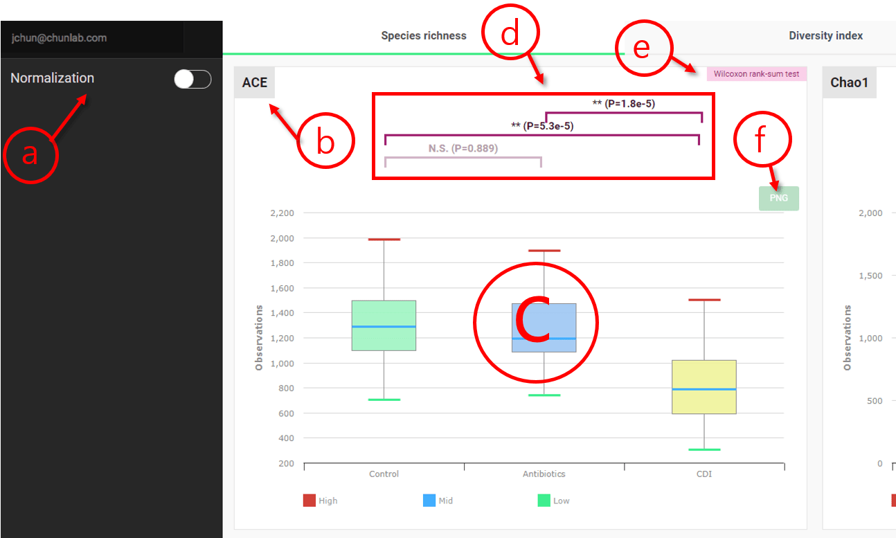
Comparing alpha-diversity in Comparative MTP Analyzer
- Apply “normalization” if you wish.
- Type of the alpha-diversity measure
- Box plots to describe the distributions among the MTP sets [Learn more]
- p-values resulted from the statistical test
- The statistical test applied (Wilcoxon rank-sum test)
- Download the chart as an image.
Beta-diversity
In this module, beta-diversity or relationship among MTPs are visualized and statistically evaluated. All calculations are based on a distance between two MTPs (microbial communities), for which several algorithms are available in EzBioCloud 16S-based MTP app.
Beta set-significance analysis
Using beta set-significance analysis, you can test if there is a significant difference between MTP sets using distance measures of beta diversity. The results are displayed in two sections. To change the types and parameters of beta diversity distance measures for this analysis, click the desired options on the left panel. The pages will be refreshed with new results instantly.
PERMANOVA results
Permutational multivariate analysis of variance (PERMANOVA), a non-parametric multivariate statistical test, is used to test the null hypothesis that the centroids and dispersion of the MTP sets as defined by measured space, are equivalent for all sets. A rejection of the null hypothesis means that either the centroid and/or the spread of the MTPs is different between the MTP sets.
PERMANOVA test is first performed with all MTP sets, then for each pair of MTP sets.
It is equivalent to the “beta-group-significance” command in the QIIME2 package.
Inter-set distances
In this visualization, beta diversity distances between a reference MTP set and a target MTP set are calculated and plotted as boxplots. When the reference set is identical to the target set, the calculations are made within a set (=intra-set distances). Otherwise, inter-set distances are calculated.
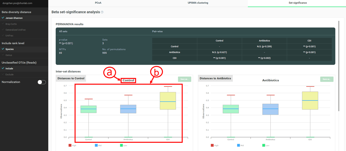
PERMANOVA results and Inter-set distances
- The reference MTP set
- The target MTP sets. In this example, MTPs in the “Control” (reference) set showed larger distances to “CDI” than “Antibiotics”. Also, the distances within “Control” and between “Control” and “Antibiotics” are similar, meaning that there is no significant difference between “Control” and “Antibiotics”. Please note that PERMANOVA test between these two sets also indicated the rejection of the null hypothesis (N.S. p=0.209).
Biomarker discovery
There are three methods for biomarker discovery. is the default method. is simple calculation of OTU presence/absence between(among) the sets. is more rigorous method than .
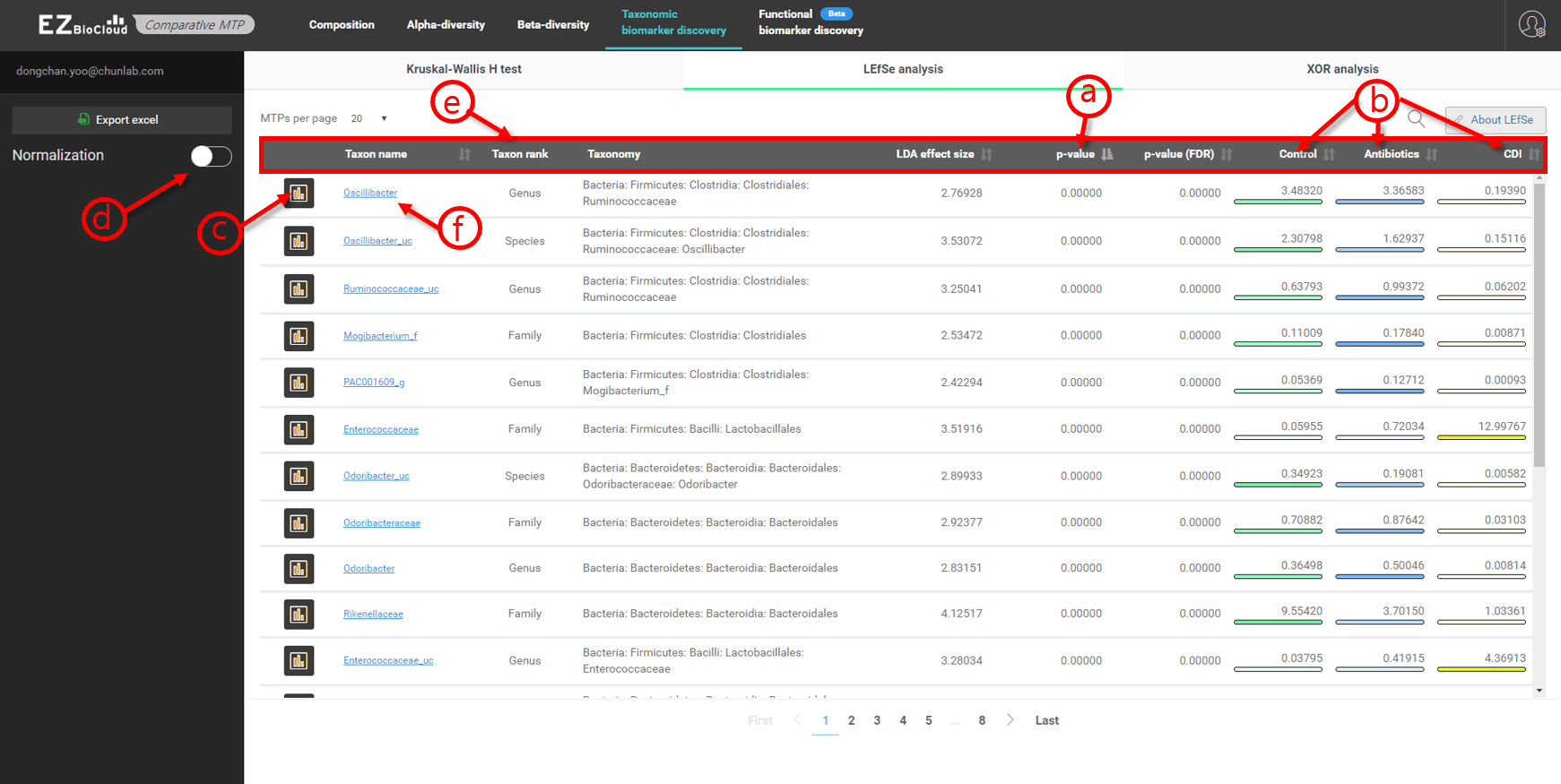
Taxonomic biomarker discovery
- Discovered biomarker taxa are listed in the order of p value.
- OTU frequencies of Control, Antibiotics and CDI sets are shown in the last three columns.
- Click to see more details on each taxon in individual bar charts or box plot.
- Apply “Normalization” function as you need.
- Click the headers to re-sort the Table.
- Click the taxon name to see the taxonomic information on EzBioCloud.
The EzBioCloud team / Last edited on Feb. 8, 2019

